Time series forecasting: When to invest for Bitcoin
Goals:
Our task in this project is to build a model with RNNs to predict bitcoin closing price the following hour given the previous 24 hours.
Here Are some questions to consider:
- Are all of the data points useful?
- Are all of the data features useful?
- Should you rescale the data?
- Is the current time window relevant?
- How should you save this preprocessed data?
Prerequisites:
- Pandas
- numpy
- tensorflow keras
- seaborn
Reference: Time series forecasting
import matplotlib.pyplot as plt
import numpy as np
import pandas as pd
import seaborn as sns
import tensorflow as tf
EDA
We start by exploring our data, in this project we have two csv files one from bitstamp and the other from coinbase, first thing first, we load the coinbase csv using pandas.
df = pd.read_csv('./data/coinbase.csv')Features
Each row in this dataframe represents bitcoin price in the given minute
- Timestamp: The unix time for each price
- Open: Opening price for each minute
- High: The Highest price for each minute
- Low: The lowest price for each minute
- Close: Closing price for each minute
- Volume_(BTC): the ammount of btc transacted in the given minute
- Volume_(Currency): the ammount of btc in USD transacted in the given minute
df| Timestamp | Open | High | Low | Close | Volume_(BTC) | Volume_(Currency) | Weighted_Price | |
|---|---|---|---|---|---|---|---|---|
| 0 | 1417411980 | 300.00 | 300.00 | 300.00 | 300.00 | 0.010000 | 3.000000 | 300.000000 |
| 1 | 1417412040 | NaN | NaN | NaN | NaN | NaN | NaN | NaN |
| 2 | 1417412100 | NaN | NaN | NaN | NaN | NaN | NaN | NaN |
| 3 | 1417412160 | NaN | NaN | NaN | NaN | NaN | NaN | NaN |
| 4 | 1417412220 | NaN | NaN | NaN | NaN | NaN | NaN | NaN |
| ... | ... | ... | ... | ... | ... | ... | ... | ... |
| 2099755 | 1546898520 | 4006.01 | 4006.57 | 4006.00 | 4006.01 | 3.382954 | 13553.433078 | 4006.390309 |
| 2099756 | 1546898580 | 4006.01 | 4006.57 | 4006.00 | 4006.01 | 0.902164 | 3614.083168 | 4006.017232 |
| 2099757 | 1546898640 | 4006.01 | 4006.01 | 4006.00 | 4006.01 | 1.192123 | 4775.647308 | 4006.003635 |
| 2099758 | 1546898700 | 4006.01 | 4006.01 | 4005.50 | 4005.50 | 2.699700 | 10814.241898 | 4005.719991 |
| 2099759 | 1546898760 | 4005.51 | 4006.01 | 4005.51 | 4005.99 | 1.752778 | 7021.183546 | 4005.745614 |
2099760 rows × 8 columns
df.isnull().sum()Timestamp 0
Open 109069
High 109069
Low 109069
Close 109069
Volume_(BTC) 109069
Volume_(Currency) 109069
Weighted_Price 109069
dtype: int64
Missing values
We notice that that we have null values in some rows, we use the fillna method from pandas with the bfill strategy (filling by previous value). i’ve used it because our missing data is at the start.
dfc=df.fillna(method="bfill")dfc.isnull().sum()Timestamp 0
Open 0
High 0
Low 0
Close 0
Volume_(BTC) 0
Volume_(Currency) 0
Weighted_Price 0
dtype: int64
Feature Selection
We notice that we have 4 columns that describe the price and 2 columns for the volume of coin, but do we need that many? As we can see, the correlation between the price features is very high this indicates that we need only the closing price.
dfcd = dfc.drop('Timestamp', axis=1)
dfcd.corr()| Open | High | Low | Close | Volume_(BTC) | Volume_(Currency) | Weighted_Price | |
|---|---|---|---|---|---|---|---|
| Open | 1.000000 | 0.999998 | 0.999997 | 0.999997 | 0.155421 | 0.393050 | 0.999999 |
| High | 0.999998 | 1.000000 | 0.999995 | 0.999998 | 0.156012 | 0.393874 | 0.999999 |
| Low | 0.999997 | 0.999995 | 1.000000 | 0.999998 | 0.154614 | 0.391870 | 0.999999 |
| Close | 0.999997 | 0.999998 | 0.999998 | 1.000000 | 0.155300 | 0.392851 | 0.999999 |
| Volume_(BTC) | 0.155421 | 0.156012 | 0.154614 | 0.155300 | 1.000000 | 0.709897 | 0.155303 |
| Volume_(Currency) | 0.393050 | 0.393874 | 0.391870 | 0.392851 | 0.709897 | 1.000000 | 0.392863 |
| Weighted_Price | 0.999999 | 0.999999 | 0.999999 | 0.999999 | 0.155303 | 0.392863 | 1.000000 |
plt.rcParams["figure.figsize"] = [7.50, 3.50]
plt.rcParams["figure.autolayout"] = True
As we can see in all the features of the price correlate visually as well.
figure, axis = plt.subplots(2, 2)
axis[0, 0].plot(dfc['Timestamp'], dfc['Open'])
axis[0, 0].set_title('Open')
axis[0, 1].plot(dfc['Timestamp'], dfc['Weighted_Price'])
axis[0, 1].set_title('Weighted Price')
axis[1, 0].plot(dfc['Timestamp'], dfc['High'])
axis[1, 0].set_title('High')
axis[1, 1].plot(dfc['Timestamp'], dfc['Low'])
axis[1, 1].set_title('Low')
plt.show()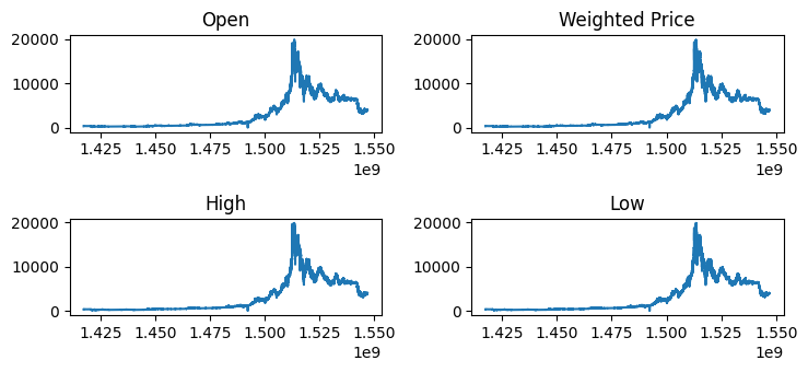
plt.plot(dfc['Timestamp'], dfc['Close'])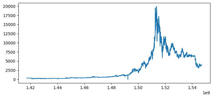
Normalization
Since the range of data goes from very low values to really high values especially with the case of the volume traded, that’s why we will implement normalization.
plt.scatter(dfc['Timestamp'], dfc['Volume_(BTC)'])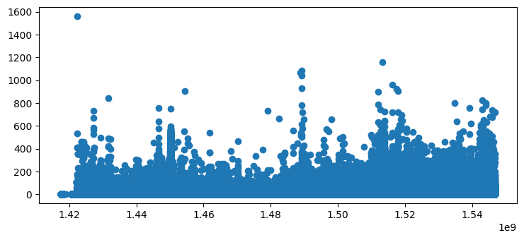
plt.scatter(dfc['Timestamp'], (dfc['Volume_(BTC)']-dfc['Volume_(BTC)'].mean())/df['Volume_(BTC)'].std())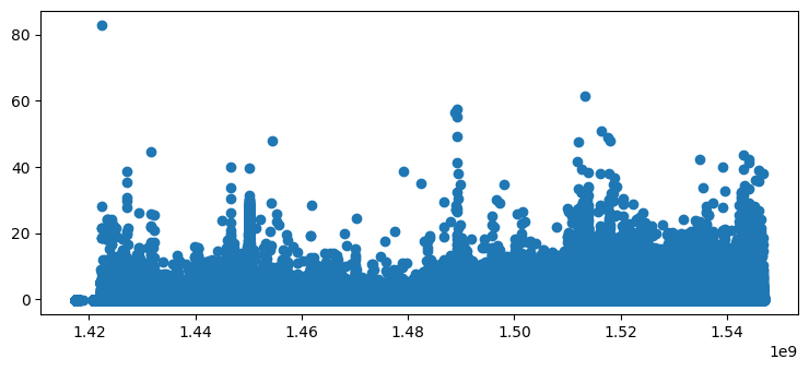
dfc.hist()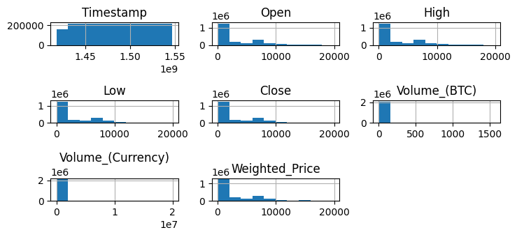
Here we imported the bitstamp data and found that it has the the same range with more values, so we will apply the same techniques and use this data instead
dfb = pd.read_csv('data/bitstampUSD_1-min_data_2012-01-01_to_2020-04-22.csv')dfb = dfb.fillna(method="bfill")dfb| Timestamp | Open | High | Low | Close | Volume_(BTC) | Volume_(Currency) | Weighted_Price | |
|---|---|---|---|---|---|---|---|---|
| 0 | 1325317920 | 4.39 | 4.39 | 4.39 | 4.39 | 0.455581 | 2.000000 | 4.390000 |
| 1 | 1325317980 | 4.39 | 4.39 | 4.39 | 4.39 | 48.000000 | 210.720000 | 4.390000 |
| 2 | 1325318040 | 4.39 | 4.39 | 4.39 | 4.39 | 48.000000 | 210.720000 | 4.390000 |
| 3 | 1325318100 | 4.39 | 4.39 | 4.39 | 4.39 | 48.000000 | 210.720000 | 4.390000 |
| 4 | 1325318160 | 4.39 | 4.39 | 4.39 | 4.39 | 48.000000 | 210.720000 | 4.390000 |
| ... | ... | ... | ... | ... | ... | ... | ... | ... |
| 4363452 | 1587513360 | 6847.97 | 6856.35 | 6847.97 | 6856.35 | 0.125174 | 858.128697 | 6855.498790 |
| 4363453 | 1587513420 | 6850.23 | 6856.13 | 6850.23 | 6850.89 | 1.224777 | 8396.781459 | 6855.763449 |
| 4363454 | 1587513480 | 6846.50 | 6857.45 | 6846.02 | 6857.45 | 7.089168 | 48533.089069 | 6846.090966 |
| 4363455 | 1587513540 | 6854.18 | 6854.98 | 6854.18 | 6854.98 | 0.012231 | 83.831604 | 6854.195090 |
| 4363456 | 1587513600 | 6850.60 | 6850.60 | 6850.60 | 6850.60 | 0.014436 | 98.896906 | 6850.600000 |
4363457 rows × 8 columns
Selecting the appropriate time range
We notice in the range of time in the data that the low range is very irrelevant (BTC at the time wasn’t as mainstream as it now) that’s why i decided to remove it out and keep the window where the ranges are relevant.
plt.plot(dfb['Timestamp'], dfb['Close'])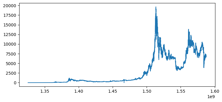
sdfb = dfb[dfb['Timestamp'] >= 1.50*1e9]Normalizing the new data
def norm(df):
return (df-df.mean())/df.std()plt.plot(sdfb['Timestamp'], sdfb['Close'])
plt.plot(sdfb['Timestamp'], norm(sdfb['Close']))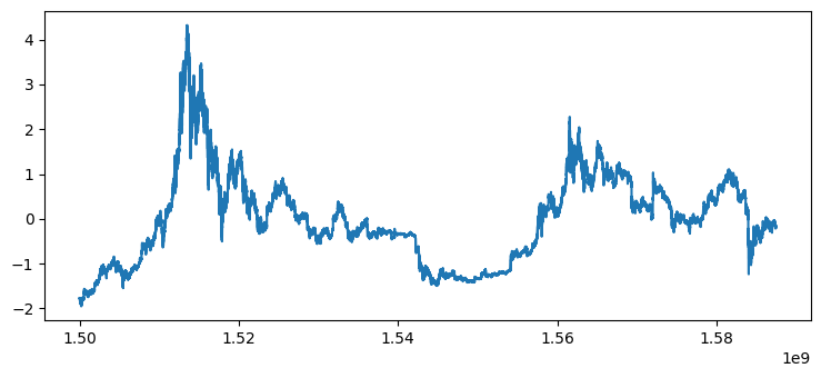
plt.scatter(sdfb['Timestamp'], sdfb['Volume_(BTC)'])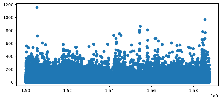
plt.scatter(sdfb['Timestamp'], norm(sdfb['Volume_(BTC)']))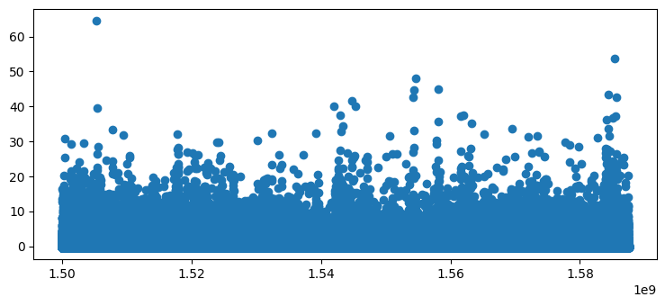
plt.scatter(sdfb['Timestamp'], sdfb['Volume_(Currency)'])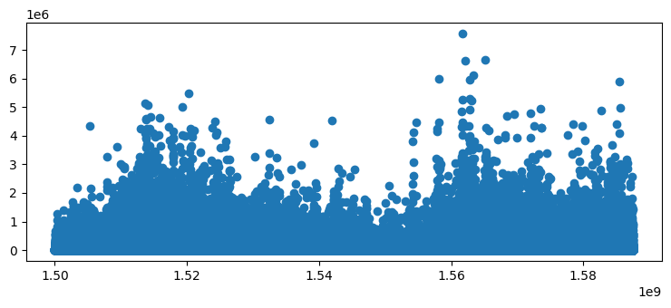
plt.scatter(sdfb['Timestamp'], norm(sdfb['Volume_(Currency)']))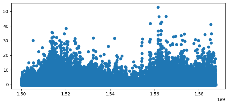
Applying feature selection on the new data
sdfb.corr()| Timestamp | Open | High | Low | Close | Volume_(BTC) | Volume_(Currency) | Weighted_Price | |
|---|---|---|---|---|---|---|---|---|
| Timestamp | 1.000000 | 0.106416 | 0.105971 | 0.107077 | 0.106404 | -0.094584 | -0.082017 | 0.106568 |
| Open | 0.106416 | 1.000000 | 0.999994 | 0.999994 | 0.999991 | 0.021313 | 0.202671 | 0.999996 |
| High | 0.105971 | 0.999994 | 1.000000 | 0.999989 | 0.999994 | 0.022329 | 0.203772 | 0.999996 |
| Low | 0.107077 | 0.999994 | 0.999989 | 1.000000 | 0.999994 | 0.020111 | 0.201358 | 0.999997 |
| Close | 0.106404 | 0.999991 | 0.999994 | 0.999994 | 1.000000 | 0.021202 | 0.202541 | 0.999996 |
| Volume_(BTC) | -0.094584 | 0.021313 | 0.022329 | 0.020111 | 0.021202 | 1.000000 | 0.914575 | 0.021153 |
| Volume_(Currency) | -0.082017 | 0.202671 | 0.203772 | 0.201358 | 0.202541 | 0.914575 | 1.000000 | 0.202488 |
| Weighted_Price | 0.106568 | 0.999996 | 0.999996 | 0.999997 | 0.999996 | 0.021153 | 0.202488 | 1.000000 |
nsdfb = sdfb.drop(['Open', 'High', 'Low', 'Weighted_Price', 'Timestamp'], axis=1)nsdfb.corr()| Close | Volume_(BTC) | Volume_(Currency) | |
|---|---|---|---|
| Close | 1.000000 | 0.021202 | 0.202541 |
| Volume_(BTC) | 0.021202 | 1.000000 | 0.914575 |
| Volume_(Currency) | 0.202541 | 0.914575 | 1.000000 |
df = nsdfb.drop(['Volume_(Currency)'], axis=1)df.corr()| Close | Volume_(BTC) | |
|---|---|---|
| Close | 1.000000 | 0.021202 |
| Volume_(BTC) | 0.021202 | 1.000000 |
df| Close | Volume_(BTC) | |
|---|---|---|
| 2904896 | 2315.97 | 1.569825 |
| 2904897 | 2315.94 | 3.100000 |
| 2904898 | 2315.97 | 1.592002 |
| 2904899 | 2315.99 | 2.091700 |
| 2904900 | 2315.97 | 0.582457 |
| ... | ... | ... |
| 4363452 | 6856.35 | 0.125174 |
| 4363453 | 6850.89 | 1.224777 |
| 4363454 | 6857.45 | 7.089168 |
| 4363455 | 6854.98 | 0.012231 |
| 4363456 | 6850.60 | 0.014436 |
1458561 rows × 2 columns
Data transformation
Since every row in our data represents a minute and we want our model to process the result from 24 hour data, we group the data by every 60 entry and we simplify the model.
df = df.groupby(np.arange(len(df))//60).mean()df.hist()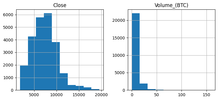
Splitting
We split our data into training, validation and testing sets for the model to train with and so we validate it
column_indices = {name: i for i, name in enumerate(df.columns)}

n = len(df)
train_df = df[0:int(n*0.7)]
val_df = df[int(n*0.7):int(n*0.9)]
test_df = df[int(n*0.9):]

num_features = df.shape[1]
train_mean = train_df.mean()
train_std = train_df.std()
train_df = (train_df - train_mean) / train_std
val_df = (val_df - train_mean) / train_std
test_df = (test_df - train_mean) / train_stddf_std = (df - train_mean) / train_std
df_std = df_std.melt(var_name='Column', value_name='Normalized')
plt.figure(figsize=(12, 6))
ax = sns.violinplot(x='Column', y='Normalized', data=df_std)
_ = ax.set_xticklabels(df.keys(), rotation=90)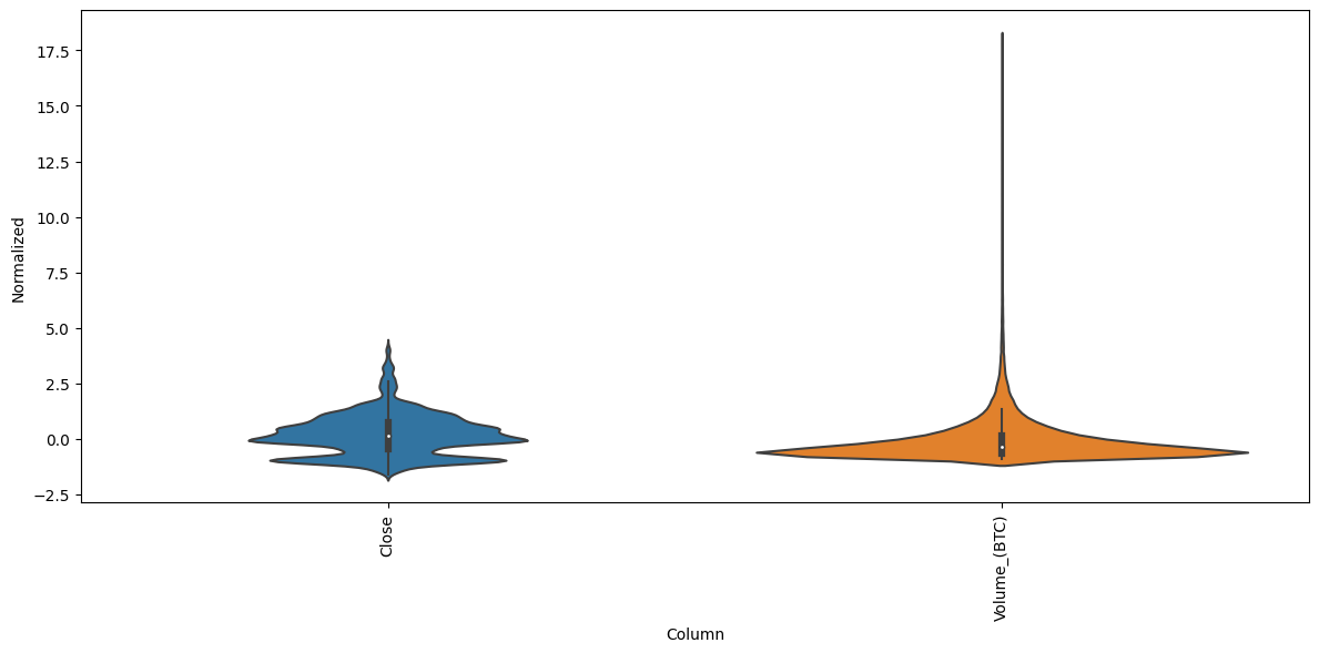
Making dataset
Tensorflow offers a very convenient api for datasets, we have a keras method to easily create a tf.data.dataset specifically for time series data with shape (batches, batch_size, sequence_length, features) after that we apply a window over the data which would split the sequence into a tuple of two sequences first element represents the past 24 hours and the other one represents the label or the next our.
def split_window(batch):
    inputs = batch[:, :24, :]
    labels = batch[:, 24, 0]
    return inputs, labels
def make_dataset(data):
data = np.array(data, dtype=np.float32)
ds = tf.keras.utils.timeseries_dataset_from_array(
data=data,
targets=None,
sequence_length=25,
sequence_stride=1,
shuffle=False,
batch_size=32)
ds = ds.map(split_window)
return dstrain_dataset = make_dataset(train_df)
val_dataset = make_dataset(val_df)
test_dataset = make_dataset(test_df)2023-01-11 14:37:35.295207: W tensorflow/compiler/xla/stream_executor/platform/default/dso_loader.cc:64] Could not load dynamic library 'libcuda.so.1'; dlerror: libcuda.so.1: cannot open shared object file: No such file or directory
2023-01-11 14:37:35.295229: W tensorflow/compiler/xla/stream_executor/cuda/cuda_driver.cc:265] failed call to cuInit: UNKNOWN ERROR (303)
2023-01-11 14:37:35.295250: I tensorflow/compiler/xla/stream_executor/cuda/cuda_diagnostics.cc:156] kernel driver does not appear to be running on this host (archpc): /proc/driver/nvidia/version does not exist
2023-01-11 14:37:35.295495: I tensorflow/core/platform/cpu_feature_guard.cc:193] This TensorFlow binary is optimized with oneAPI Deep Neural Network Library (oneDNN) to use the following CPU instructions in performance-critical operations: AVX2 FMA
To enable them in other operations, rebuild TensorFlow with the appropriate compiler flags.
train_dataset.save('./datasets/train')
val_dataset.save('./datasets/val')
test_dataset.save('./datasets/test')
Modeling,Training and Evaluation
For modeling we will be using tensorflow keras, but first we need to create a tensorflow.data.dataset object for our RNN to consume, we also perform splitting on the dataset to make it into a tuple of (inputs, prediction) with the input being 24 time sequences (24 hours) and prediction being 1 time sequence (1 hour).
lstm_model = tf.keras.models.Sequential([
    # Shape [batch, time, features] => [batch, time, lstm_units]
    tf.keras.layers.LSTM(32, return_sequences=False),
    # Shape => [batch, time, features]
    tf.keras.layers.Dense(units=1)
])
def compile_and_fit(model, train, val, epochs=20, patience=2):
early_stopping = tf.keras.callbacks.EarlyStopping(monitor='val_loss',
patience=patience,
mode='min')
model.compile(loss=tf.keras.losses.MeanSquaredError(),
optimizer=tf.keras.optimizers.Adam(),
metrics=[tf.keras.metrics.MeanAbsoluteError()])
model.fit(train, epochs=epochs,
validation_data=val,
callbacks=[early_stopping])As we can see early stopping stopped the training when it converged
compile_and_fit(lstm_model, train_dataset, val_dataset)Epoch 17/20
532/532 [==============================] - 6s 11ms/step - loss: 0.0018 - mean_absolute_error: 0.0221 - val_loss: 0.0013 - val_mean_absolute_error: 0.0193
Evaluation
We will visually evaluate the model by plotting some examples and their predictions.
example_window = tf.stack([np.array(test_df[:25]),
                           np.array(test_df[100:100+25]),
                           np.array(test_df[200:200+25])])
example, _ = split_window(example_window)
predictions = lstm_model.predict(example)1/1 [==============================] - 0s 414ms/step
predictionsarray([[0.45651057],
[0.64009064],
[0.6150275 ]], dtype=float32)
def unormalize_res(df):
    return df * train_std[0] + train_mean[0]
pred = unormalize_res(predictions[0])
exp = unormalize_res(np.array(test_df[:25])[:, 0])
plt.scatter(list(range(25)), exp)
plt.scatter([24], pred)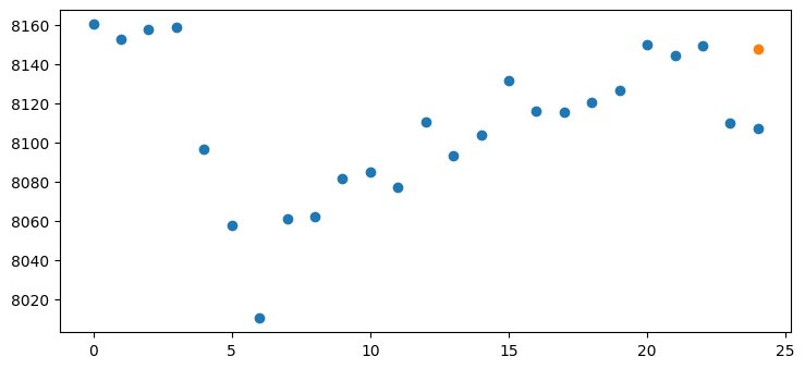
pred = unormalize_res(predictions[1])
exp = unormalize_res(np.array(test_df[100:100+25])[:, 0])
plt.scatter(list(range(25)), exp)
plt.scatter([24], pred)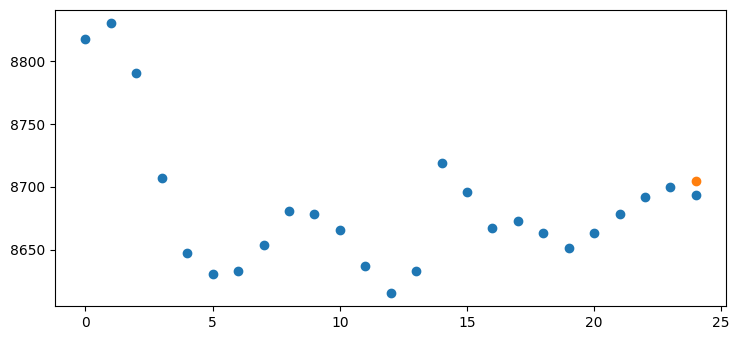
pred = unormalize_res(predictions[2])
exp = unormalize_res(np.array(test_df[200:200+25])[:, 0])
plt.scatter(list(range(25)), exp)
plt.scatter([24], pred)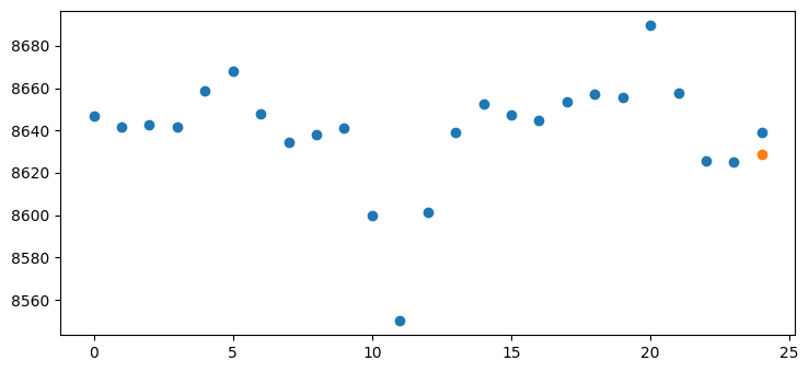
Conclusion
As we know bitcoin predictability is very low as it is very linked to other trends such as social media, inflation and overall news, but from our random examples we get overall good results, we can do use a smaller time frame or acquire more data and add more features such as bitcoin sentiment and inflation.