Optimization

Optimization Methods in ML

Different gradient descent optimization methods

What is optimization?

Optimization deals with techniques to get better training results during back-propagation. We won’t be covering hyper-parameter optimization rather training optimization, These are the techniques we will be covering in this article:

• Feature Scaling
• Mini-batch gradient descent
• Batch normalization
• Gradient descent with momentum
• Learning rate decay
• RMSProp optimization
• Adam optimization

Feature Scaling

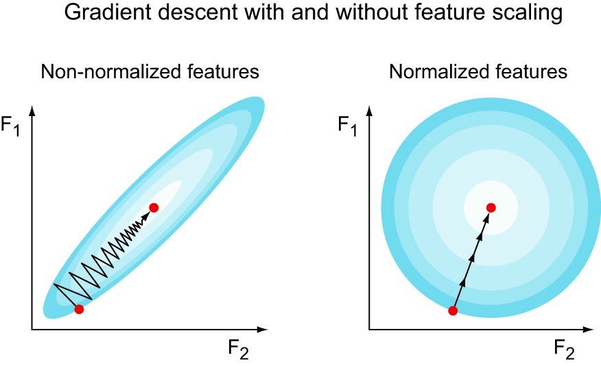
Feature scaling is a method used to normalize the range of independent variables or features of data. It is also known as data normalization.

Since the range of values of raw data varies widely,objective functions will not work properly without normalization.

One of the methods of feature scaling is Standardization (Z-score Normalization):

norm_x = x-avg(x)/stddev(x)

Feature standardization makes the values of each feature in the data have zero-mean (when subtracting the mean in the numerator) and unit-variance. This method is widely used for normalization in many machine learning algorithms The general method of calculation is to determine the distribution mean and standard for each feature. Next we subtract the mean from each feature. Then we divide the values (mean is already subtracted) of each feature by its standard deviation.

Mini-Batch Gradient Descent

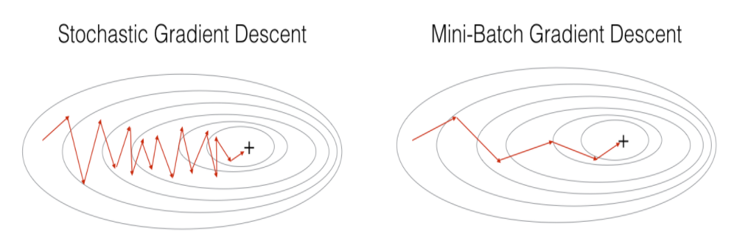
Mini-batch gradient descent is a variation of the gradient descent algorithm that splits the training dataset into small batches that are used to calculate model error and update model coefficients.

Mini-batch gradient descent seeks to find a balance between the robustness of stochastic gradient descent and the efficiency of batch gradient descent. It is the most common implementation of gradient descent used in the field of deep learning.

• The model update frequency is higher than batch gradient descent which allows for a more robust convergence, avoiding local minima.
• The batched updates provide a computationally more efficient process than stochastic gradient descent.
• The batching allows both the efficiency of not having all training data in memory and algorithm implementations.

Batch normalization

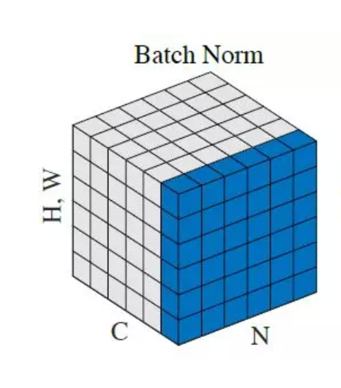
For each feature, batch normalization computes the mean and variance of that feature in the mini-batch. It then subtracts the mean and divides the feature by its mini-batch standard deviation. Resulting in transforming the inputs to be mean 0 and unit variance.

is a technique for improving the speed, performance, and stability of artificial neural networks. It is used to normalize the input layer by adjusting and scaling the activations.

We apply a batch normalization layer as follows for a minibatch B:

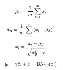
where omega and beta are a learnable parameter.

Gradient descent with momentum

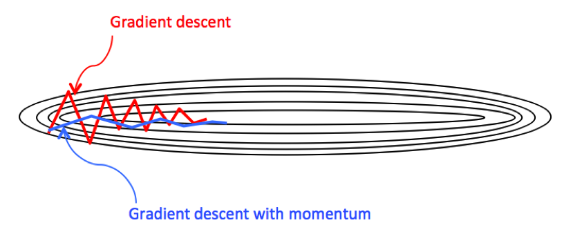
Gradient descent with momentum seeks to decrease the oscillation in gradient descent and in turn make more step towards the global minimal by using momentum to normalize the step towards it, This is what called in statistics as moving average.

Imagine you have a ball rolling from point A. The ball starts rolling down slowly and gathers some momentum across the slope AB. When the ball reaches point B, it has accumulated enough momentum to push itself across the plateau region B and finally following slope BC to land at the global minima C.

Learning rate decay

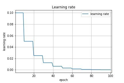
Learning rate decay is a technique in Deep learning where the we tune the learning as the learning progress as the name suggests the learning rate decays aka. goes down as as we train more epochs like the visual above.

A common learning rate decay formula goes as follows:

“ α=(1/(1+decayRate×epochNumber))*​α0 ”

1 epoch : 1 pass through data

α : learning rate (current iteration)

α0 : Initial learning rate

decayRate : hyper-parameter for the method

We use learning rate decay to avoid oscillation in gradient descent and thus avoid early convergence to a local minima.

RMSProp

Root Mean Squared Propagation, or RMSProp for short, is an extension to the gradient descent optimization algorithm.

RMSProp is designed to accelerate the optimization process, e.g. decrease the number of function evaluations required to reach the optima, or to improve the capability of the optimization algorithm, e.g. result in a better final result.

It is related to another extension to gradient descent called Adaptive Gradient, or AdaGrad.

AdaGrad is designed to specifically explore the idea of automatically tailoring the step size (learning rate) for each parameter in the search space. This is achieved by first calculating a step size for a given dimension, then using the calculated step size to make a movement in that dimension using the partial derivative. This process is then repeated for each dimension in the search space.

Adam

Adam is an optimization algorithm that can be used instead of the classical stochastic gradient descent procedure to update network weights iterative based in training data.

The authors describe Adam as combining the advantages of two other extensions of stochastic gradient descent. Specifically:

• Adaptive Gradient Algorithm (AdaGrad) that maintains a per-parameter learning rate that improves performance on problems with sparse gradients (e.g. natural language and computer vision problems).
• Root Mean Square Propagation (RMSProp) that also maintains per-parameter learning rates that are adapted based on the average of recent magnitudes of the gradients for the weight (e.g. how quickly it is changing). This means the algorithm does well on online and non-stationary problems (e.g. noisy).

Adam realizes the benefits of both AdaGrad and RMSProp.

Instead of adapting the parameter learning rates based on the average first moment (the mean) as in RMSProp, Adam also makes use of the average of the second moments of the gradients (the uncentered variance).

Specifically, the algorithm calculates an exponential moving average of the gradient and the squared gradient, and the parameters beta1 and beta2 control the decay rates of these moving averages.

The initial value of the moving averages and beta1 and beta2 values close to 1.0 (recommended) result in a bias of moment estimates towards zero. This bias is overcome by first calculating the biased estimates before then calculating bias-corrected estimates.

Conclusion

Optimization is a wide subject that’s still researched today with different methods popping up everyday, all for the same objective to make learning faster and more precise (convergence to global minima).

Next time we will discuss Regularization.